Contrastive Learning

Suppose you have a lot of unlabeled data and you want to train your model on it, for these kind of tasks we use SSL (Self Supervised Learning). This makes a model learn from the unlabeled data without having labels for it.

Contrastive learning is one of the techniques in SSL, that makes our model learn from the unlabeled data.

Cost functions

As the name suggests contrastive learning learns by “contrasting” between the examples (which are actually vectors), now our goal is to make our model learn that similar examples are similar and non similar ones are not. We do this by having cost functions that serve this purpose, since our goal is to always minimize the cost function we should make cost functions that calculate the errors in our predictions. I am sharing 2 cost functions below.

Triplet loss

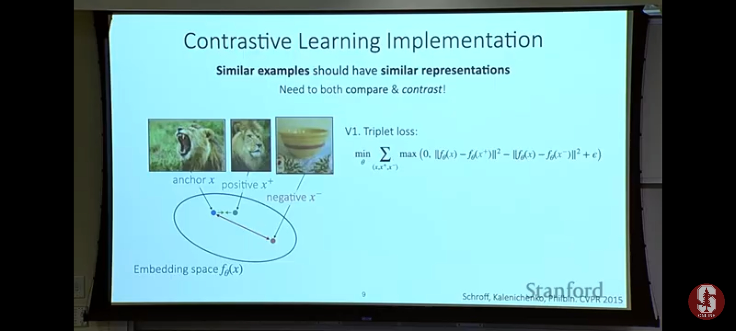
In calculating triplet loss we have only 3 things, anchor: the image we want our model to learn about, positive image: another similar image to the anchor, can be a little different because we apply transformations on the anchor to get this, so model is forced to learn the deep similarities between the anchor and positive image, negative image: a different image which is not similar to the anchor, it’s best to use image which looks almost similar to the anchor but is actually different this forces our model to learn deep representations rather than shallow.

The reason we are subtracting these L2 norms and then taking the max() with 0, is to prevent negative loss which will come if our model learns very well that our negative image is different and places it very far on the embedding space. Then we obviously use summation to sum all the losses over all the examples.

NT-Xent loss

This is quite different from triplet loss, we compare one example with multiple different examples, this makes the model learn how one example differs from all the others. In general we compare an example with all the other examples and note down how much similar our example is to the other examples. If we have N examples then each example will be compared with N examples (including itself) which gives us N*N values in total, and we can form a nice matrix out of it, where similarity of one example with all the N examples (including itself) is in the row format.

One cool thing that you can notice about this matrix is that all the values on it’s columns are 1 which is because at those indices each example is being compared with itself, suppose we have examples named as v1,v2,………,vm, then each value of each vi is 1 at the ith column as it’s being compared with itself. When I say compared it just means that we are using some method to calculate the similarity between the examples which are just encoded vectors.

That was all for this week!