What I learnt by Building a Neural Net from Scratch

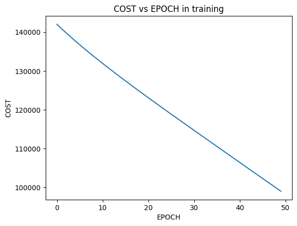
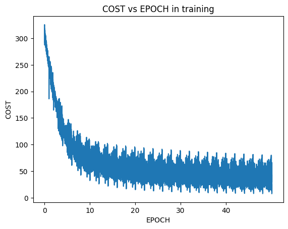
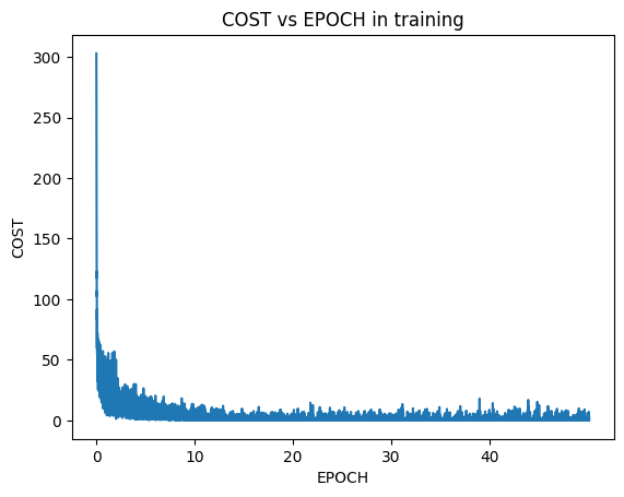
I went from 0 to 97% accuracy on test set on a Neural Net that I built from Scratch. Here are the performance using various algorithms:
So I have been working on building a neural net from scratch in the couple of weeks and I have learnt a lot of new things.
I used to think that building a Neural net is pretty hard but it’s not actually that hard if you really sit down and scratch your head a lil bit you will eventually build one just like me.
At first I thought, “this is it I have built it” but then some error comes or outputs are not as you expect or training takes a lot of time and all those small problems arise from somewhere. Then you find yourself in Problem - Solve loop where you are basically solving the problems that are coming after solving the previous one.
Basic structure of a neural net is simple: Input -> Layers -> Output. Structure of processes: Input -> Forward prop -> Compute cost or store it -> Backward prop -> Gradient Descent -> Repeat until epochs are compelte or you reach your goal.
BUILDING THE BASIC ELEMENTS
In this section we will build all the basic elements required to build a neural net from scratch. This includes: Forward prop, Backward prop, Train and a Prdict function. A perameter initialization function.
Here is a simple analogy to think of Neural Nets.
You can think of a neural network as something like a factory where you put raw potatoes (data) in and chips (output) comes out. It’s obvious that those potatoes have gone through a lot of hidden processing in the factory (neural net). And we go through this cycle (forward prop) again and again until we produce the chips that are one of the best.
To produce the best chips we need a standard to compare themselves against and that standard is the best chips in the city (output values of input matrix, y).
Forward Propagation
Forward prop and forward propagation are the same if you are confused about that.
So, why do we need forward prop? The reason is simple. You want your model to learn from the underlying data patterns, each layer of the neural network learns something different about the data. That’s why you pass the data ahead in the network.
The output layer of the network generally outputs the type of output (generally vectors and matrices) that matches the output labels with the training data, so that computing the accuracy of our predictions becomes easy, and this is the right way to do it.
In this section I am going to specifically talk about the forward pass for neural networks.
Forward pass in case of Neural Networks is quite different than that of some simple linear model, when you do forward pass in the neural network you go on storing activation values and the outputs of different layers in cache (some kind of memory, don’t know much about it now :p).
When I first learnt about it I though why we are even doing this why it’s not that simple, but since we are building a neural net so we can expect such hard things to come along our way.
As the data flows ahead in the neural net, each layer gives it’s output which is based on the input from the previous layer. In this sense first layer gets it’s inputs from the input matrix itself (also called input layer or layer 0).
Each layer computes Z’s and activation values, and we are going to store them as we will need them for backprop. We usually store them in a dictionary, I am doing the same in my project.
We are not done when the output comes out of the network because we are not sure if it is the right output or the model is learning the right things or if the perameters model has learnt are right. We need to improve our perameters as our output is the result of those perameters.
To make sure how much accurate we are, we compute a loss function. The simple idea behind computing a loss function is to know how much total error our predictions have.
The loss function evaluates how far the model’s predictions are from the true values. We compute the loss for each example and average them to guide the model’s learning.
There are a lot of loss functions depending upon the task you are into, some of the common ones are: mean squared loss, binary cross entropy, cross entropy etc.
- Mean Squared Loss: This is a simple cost function. The idea is that you plot your predictions and true values on a plane, find the difference between predicted value and true value for some input, square this difference and then take average of that. That is why it is “mean” of losses that are squared.
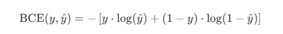
- Binary Cross Entropy: This function is used if you are dealing with the tasks where you need to predict out of two available classes which class the example belongs to, that just means for binary classification tasks. It is generally used with sigmoid which is also used for binary classification tasks.
There are a lot of other cost functions and we will talk about them some other time.
Backward Propagation
Let’s talk about back prop a little bit. The reason that we need backprop is that with the weights and biases that our models have initially, we might not be able to make the best predictions because they are initialized randomly; it’s almost always the case that our predictions are far from the best.
So, we need some method that, if not at once, eventually takes us to the right weights and biases; backpropagation is for exactly that.
The overall idea of backprop is that it makes the parameters of our network better and better with each iteration. First initialization might not be the best, but when you make the 100th update to those parameters using this algorithm, then you will have better weights and biases that make better predictions than your first initialized variables.
These fundamental ideas will help us build our neural network and you will be able to see how these ideas are being used in our code.
Back To Code
We will start by importing the basic libraries needed to build this network.
import numpy as np
import matplotlib.pyplot as plt
import time
These are just simple libraries that we will need to build our network. Also (a little bit of Philosophy), that a neural net is a mathematical function, you can break a neural net into a computational graph and think of it as just a function that is just performing matrix manipulations.
Generally, we try to write code for a neural net inside the class so we can make a lot of instances of it, so keep a basic template of a class ready to fill it up with code for a neural net.
class l_layer_NN():
	def __init__(self):
		pass #code here
Forward Propagation Code
As described above neural net goes through repeated forward and backpropagations, so this is the part of forward propagation.
Forward propagation involves doing calculations using the equation below:
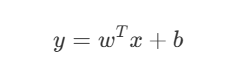
Now, let’s focus on the first part of the matrix, which is the weight matrix (W). We want a function that will initialize weight matrices for us in such a way that they are suitable for the dimensions of our data.
Then we will store these matrices somewhere, which are just weights and biases of each layer, and improve them with each iteration to give us more accurate predictions. We don’t want to initialize these matrices again and again at the start of each iteration; that’s why we save them somewhere.
Since we are building a neural net with multiple layers, each layer will have its own weight matrix. You might know that each layer in a neural network generally contains more than 1 perceptron, and each perceptron is just a simple calculation unit that gives us a linear relation based on the weight matrix that it has. This also means that each perceptron has its own weight matrix.
The weight matrix of any layer in a neural network is formed from the weight matrices of these perceptrons. Specifically, the rows of the weight matrix of a layer are the transposes of the weight matrices of the perceptrons in that layer.
Now, if we have a simple 5-layer neural network, then there will be 5 weight matrices belonging to each layer of the network, and each one of them has the “mini” weight matrices of the layer they belong to.
Here is the simple code to initialize weight matrices for each layer before forward propagation, because if you don’t do it, I don’t know what you will multiply your inputs with.
  def params_ini(self,X):

    for i in range(len(self.layer_units)):
      if i == 0:
        self.params[f"W{i+1}"] = np.random.randn(self.layer_units[0],X.shape[0]) * np.sqrt(2/X.shape[0]).astype(np.float32)
        self.params[f"b{i+1}"] = np.zeros((self.layer_units[i],1)).astype(np.float32)

      else:
        self.params[f"W{i+1}"] = np.random.randn(self.layer_units[i], self.layer_units[i-1])  * np.sqrt(2/self.layer_units[i-1]).astype(np.float32)
        self.params[f"b{i+1}"] = np.zeros((self.layer_units[i],1)).astype(np.float32)
By looking at this code, we can tell that there is some difference between the first layer and all the other layers of the network. That difference is simple: the columns of the weight matrix are equal to the rows of the input matrix because of the simple matrix multiplication rule.
The idea of forward propagation is simple: to produce the outputs by passing inputs through each layer until they reach the final layer and come out.
That’s what will happen: you put the inputs into the network, each layer calculates its outputs, passes that as input for the next layer, and the next layer does the same until you have your output. The following code does the same:
  def forward_prop(self, X):

    out = X
    self.forward_cache["A0"] = X
    L = len(self.layer_units)

    for i in range(1,L+1):
      W = self.params[f"W{i}"]
      b = self.params[f"b{i}"]
      Z = W @ out + b
      A = (self.hidden_activ(Z) if i!=len(self.layer_units) else self.final_l_activ(Z))

      self.forward_cache[f"Z{i}"] = Z
      self.forward_cache[f"A{i}"] = A
      out = A

    return out
The code does the same as described above. We calculate the output of each layer using a for loop and then apply th activation function to it and store it in A.
You might also notice that we are storing values of Z and A in forward_cache. We are storing these values in cache as they will be needed in the backpropagation step.
In the end this code returns the output of the last layer and we are only concerned with it!
Cost Function
Cost function are used to evaluate our model’s performance. After making predictions it’s a reasonable step to figure out how much accurate they are, we do this by using a cost function.
A cost function can differ depending upon the variety of the task we are working on. In my project I have included on two types of cost functions but there can be more. The code below computes the total cost of the predictions of the model.
  def loss_compute(self,y_pred,y):

    m = y.shape[1]

    if self.final_activ=="sigmoid":
      y_pred = np.clip(y_pred,self.epsilon,1-self.epsilon)
      cost = -np.sum(y*np.log(y_pred + self.epsilon) + (1-y)*np.log(1 - y_pred + self.epsilon)) / m

    else:
      cost = -(1/m) * np.sum((y * np.log(y_pred)))

    return cost
This function takes in the predictions made by the model and the actual target values for the inputs. I have made this only for two type of tasks classification (sigmoid) and regression. The last function computes cost on regression tasks and first one on classification tasks.
Now it’s time to go backward, that is to say use backpropagation to calculate gradients in order to make our model weights able to give us better predictions.
Backpropagation
Here is the code I used for backpropagation:
  def back_prop(self, y):

    m = y.shape[1]

    dA = self.forward_cache[f"A{int(len(self.forward_cache)/2)}"] - y
    self.grads["dA"] = dA

    for l in range(int(len(self.forward_cache)/2),0,-1):
      dA = self.grads["dA"]
      if l == int(len(self.forward_cache)/2):
        if self.final_activ == "sigmoid":
          dZ = dA * self.forward_cache[f"A{l}"] * (1-self.forward_cache[f"A{l}"])
        else:
          dZ = dA

      else:
        dZ = dA * (self.forward_cache[f"Z{l}"] > 0)

      dW = (1/m) * dZ @ self.forward_cache[f"A{l-1}"].T
      db = (1/m) * np.sum(dZ,axis=1, keepdims=True)
      dA_prev = self.params[f"W{l}"].T @ dZ

      self.grads[f"dW{l}"] = dW
      self.grads[f"db{l}"] = db
      self.grads["dA"] = dA_prev
At first it looks liks a mammoth but it’s actually pretty simple, for this you need to understand backpropagation. Many people are afraid of backpropagation, so I try to explain this here simply.
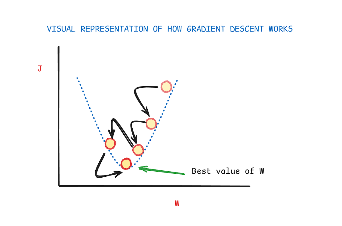
In backpropagation, you are generally concerned with calculating the gradient of each component of the neural network, then, with the help of the gradient for some particular parameter, you push it in the right direction in such a way that you reduce its overall contribution to the total cost.
This idea is quite similar to the simple gradient descent that we use in linear and logistic regression. We need these gradients because of our optimization function. Mostly, we use gradient descent as our optimization function, and it requires us to calculate gradients, which is why we calculate them. I have used other optimization algorithms like ADAM, also I will also explain them in the end.
At first, we start by calculating how the activations of the final layer affect our outputs; for that, we use the simple calculus we used in high school. But we have to keep in mind that this derivative can change depending on the task or loss function you are using.
Let’s say you are working on a regression task, and we have a cost function that looks like below.

We are using 2 in the denominator here because this will make our calculations easy.
Now we have to calculate the gradient of the cost function with respect to the activation values of the final layer. On doing so, we get these values:
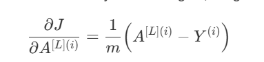
Here, A is the final layer activations and we are using the cost function given above.
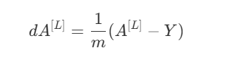
Using 2 in the denominator helped cancel the exponent 2 that came out by differentiating. But we are not done yet. To make our calculations faster, we need to vectorize our calculations. You might know that vectorization helps speed up our calculations.
I think this is because vectorization reduces the total number of steps you have to get to the final result of your calculations. So the vectorized formula from above turns into this:
Now we have an expression that tells us how activations of the final layer make changes to the overall cost function of the model. But we need to trace it back even further in order to find out how the weights of our model impact the final cost.
Let’s find out how Z of the final layer impacts the cost function. At first, when you write out the expression, you can’t figure out how exactly this impact the final output, but we can break this into activations of the final layer, because A is just the function of Z, and we can take the help of our beloved chain rule.
This is the vectorized version of how the vector Z of the final layer impacts the cost function.
This is also called the loss of the layer and is denoted by delta[L] (last layer), for simple hidden layers it’s delta[l]. Now we are closer to finding how the weights of the final layer impact the cost function.
Here, we can use our little brain to think about it and find the derivative of J wrt W of the last layer. We know that W affects Z and Z affects A, so we can actually break this dJ/dW derivative down into the derivative of Z and A. That’s what we do below, it’s just the simple chain rule.
But to improve our network fast, we don’t just need to find the derivative of the cost function with respect to the final layer, but we need to find it for all the weight matrices of each layer in the network, so that each layer will give us a better output.
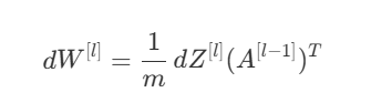
The code below calculates all the gradients that are required to use optimization functions on each parameter.
  def back_prop(self, y):

    m = y.shape[1]

    dA = self.forward_cache[f"A{int(len(self.forward_cache)/2)}"] - y
    self.grads["dA"] = dA

    for l in range(int(len(self.forward_cache)/2),0,-1):
      dA = self.grads["dA"]

      if l == int(len(self.forward_cache)/2):
        if self.final_activ == "sigmoid":
          dZ = dA * self.forward_cache[f"A{l}"] * (1-self.forward_cache[f"A{l}"])
        else:
          dZ = dA

      else:
        dZ = dA * (self.forward_cache[f"Z{l}"] > 0)

      dW = (1/m) * dZ @ self.forward_cache[f"A{l-1}"].T
      db = (1/m) * np.sum(dZ,axis=1, keepdims=True)
      dA_prev = self.params[f"W{l}"].T @ dZ

      self.grads[f"dW{l}"] = dW
      self.grads[f"db{l}"] = db
      self.grads["dA"] = dA_prev
The for loop in this code goes from the last layer to the 1st layer. I have used here int(len(self.forward_cache)/2) which is not a good practice, but let’s get ahead with that for now. self.forward_cache contains all the activations and Z’s we have stored for each layer, since each layer has one activation value as output (A) and Z, so the length of self.forward_cache is 2 times the number of layers in the network, that’s why I divided it by 2 there.
When you look at this part of the code:
      if l == int(len(self.forward_cache)/2):
        if self.final_activ == "sigmoid":
          dZ = dA * self.forward_cache[f"A{l}"] * (1-self.forward_cache[f"A{l}"])
        else:
          dZ = dA
You will find that dZ for the last layer changes depending upon the activation function of the last layer we have chosen. We do this because activation function of the last layer needs to be changed depending on the task we are working with. In my code, I have only 2 activation functions, one for the classification task (sigmoid) and the other one is softmax (I guess!).
The rest of the code below calculates gradients for the process as mentioned above.
Optimization Functions
After calculating the gradients our next task is to update our perameters using those gradients. This is very important because the choice of the opcimization function can either make your performance worse or improve it a lot.
Generally we use a simple optimization function like Gradient Descent to do this. This is the code I have used in my model, this goes layer by layer, starting from the first layer to the final layer. Notice I have used self.use_adam in the if condition, ADAM is also an optimizer function, this is very fast than just simple Gradient Descent algorithm. It improves the performance of GD a lot. I am not going into the mathematical aspects of how ADAM does this (i need to learn more about it) but still below is the code for both of them.
The simple function of an optimizer function is to make changes to the model perameters so that it gives us more accurate outputs, these activation function do the same. Also, notice that ADAM function below just returns a dictionary with some values and not updating the perameters like gradient descent function, this is because we are using ADAM inside gradient descent function, that’s why there is self.use_adam there, so when we want to use ADAM optimizer, self.use_adam is set to True.
  def gradient_descent(self):

    self.t += 1
    if self.use_adam:
        adam_res = self.adam()

    for l in range(1,int(len(self.params)/2)+1):

      if self.use_adam:
        self.params[f"W{l}"] -= (self.l_rate * adam_res[f"WFM{l}"]) / (adam_res[f"WSM{l}"] + self.epsilon)
        self.params[f"b{l}"] -= (self.l_rate * adam_res[f"BFM{l}"]) / (adam_res[f"BSM{l}"] + self.epsilon)

      else:
        self.params[f"W{l}"] -= (self.l_rate*self.grads[f"dW{l}"])
        self.params[f"b{l}"] -= (self.l_rate*self.grads[f"db{l}"])
def adam(self):


    n_layers = len(self.layer_units)
    t = self.t

    adam_res = {}

    for i in range(n_layers):
      dW,db = self.grads[f"dW{i+1}"], self.grads[f"db{i+1}"]

      self.m_m[i+1] = self.beta1 * (self.m_m[i+1]) + (1-self.beta1) * (dW)
      self.v_m[i+1] = self.beta2 * (self.v_m[i+1]) + (1-self.beta2) * (dW**2)

      self.m_b[i+1]  = self.beta1 * (self.m_b[i+1]) + (1-self.beta1) * (db)
      self.v_b[i+1] = self.beta2 * (self.v_b[i+1]) + (1-self.beta2) * (db**2)

      m_m_hat = self.m_m[i+1] / (1-self.beta1**t)
      v_m_hat = self.v_m[i+1] / (1-self.beta2**t)

      m_b_hat = self.m_b[i+1] / (1-self.beta1**t)
      v_b_hat = self.v_b[i+1] / (1-self.beta2**t)

      adam_res[f"WFM{i+1}"] =  m_m_hat
      adam_res[f"WSM{i+1}"] =  v_m_hat
      adam_res[f"BFM{i+1}"] =  m_b_hat
      adam_res[f"BSM{i+1}"] =  v_b_hat


    return adam_res
Now that we have included forward prop + backward prop + loss function in our model, and some optimization functions, we need to train make some functionality that allows our model to be trained.
Training loop of a model is pretty simple: Forward prop –> Compute Loss –> Backward Prop –> Optimization. We go through this loop many times, generally you fix it beforehand how many times you want to go through the loop. The code below is the training loop of the model:
 def train(self,X,Y):

    self.params_ini(X)
    a = time.time()
    for epoch in range(self.epochs):

      if self.mini_batch:
          self.train_mini_batch(X,Y, epoch, True)

      else:
        y_preds = self.forward_prop(X)
        cost = self.loss_compute(y_preds, Y)
        self.costs.append(cost)
        self.back_prop(Y)
        self.gradient_descent()
Notice we are using something called self.train_mini_batch, this is called using mini batches. Mini batches just means that instead of putting all of your data at once into the model you do it in chunks, one by one.
This prevents overfitting that is instead of learning the underlining patterns of the data model learns the data itself and as a result starts performing poorly on new data. When using mini batch we make updates in the model patameters after each mini batch, while before when we were putting whole data as a single batch we used to make a single change for a single pass through the whole data. So using mini batches increases the number of updates you make to your perameters and as a result improves the model performance.
def train_mini_batch(self,X,Y, epoch, even_shuffle = False):

    m = X.shape[1]

    if even_shuffle and epoch%2==0:
      perm = np.random.permutation(m)

      X_shuffled = X[:, perm]
      Y_shuffled = Y[:, perm]
      batches = self.create_mini_batches(X_shuffled,Y_shuffled)

    else:
      batches = self.create_mini_batches(X,Y)

    for i in range(len(batches)):

      out = self.forward_prop(batches[i][0])
      cost = self.loss_compute(out,batches[i][1])
      self.costs.append(cost)
      self.back_prop(batches[i][1])
      self.gradient_descent()
Notice we are using, perm = np.random.permutation(m) which helps in randomizing the rows in each batch, so for every new pass through the data each batch will have different rows than what it had before.
This helps model in learning the underlining pattern of the data instead of learning the data itself.
To predict the output of the data we need this function below:
  def predict(self, X):

    m = X.shape[0]
    X = X.T.reshape(-1,m)

    return self.forward_prop(X)
So, on calling model.predict() we will just get our outputs.
I have used the code from this repo. You will find more useful functions and an overall big picture of model here.
Thanks for reading!